The numbers you memorised were a distribution

Every engineer carries the same little table of latency constants: memory is ~100 ns, an SSD read is ~16 µs. We quote them like physical constants. But each entry was only ever the centre of a wide, drifting distribution, measured on particular hardware in a particular year — a point estimate wearing the costume of a fact.

I’ve quoted a latency number from memory in the past. “Main memory is about a hundred nanoseconds, so keeping the hot set in-process buys a couple of orders of magnitude over the round trip,” and nobody evers blinks, because every other software engineer has the same table in their head. It’s the “numbers every programmer should know” table, or one of its descendants; Dan Luu spent part of a recent benchmarking post poking at the napkin-math version of it, asking whether the constants are actually right. I read that expecting to nod along, and instead got a little uncomfortable, because I realised I’d been treating those numbers the way I treat the speed of light.

That table is one of the those useful things I own. It lets me rule out a design in my head before I’ve written a line — if the plan needs a million disk seeks on the request path, I already know it’s dead without benchmarking it — and it lets a room full of engineers reason about orders of magnitude in a shared language. The reflex it trains, though, is to read each figure as a property of the hardware: a memory reference simply is a hundred nanoseconds, the way an electron simply has the charge it has. That reflex is mine by default, and it’s the one I need to slow down.

A constant that was always a measurement

A memory reference is not a hundred nanoseconds. It’s around a hundred nanoseconds when the line is where you hoped, more when it isn’t, more again under contention, more still across a NUMA boundary or when the prefetcher guessed wrong. The single figure I carry is a central tendency — a mean, or something near the median — with the whole spread cropped out of frame. It’s a point estimate, but I’ve been reading it as though the spread were zero.

What’s odd is that I already distrust this everywhere else. I’d never accept “the endpoint takes 40 ms” as a statement about the endpoint; my first question is under what load, because I know perfectly well that latency is a response to conditions and not a scalar the code carries around in its pocket. Load testing exists precisely because nobody sane believes a single latency number — you drive the thing across a range of conditions and look at the curve that comes back. Somehow the numbers in my head had been exempted from the suspicion I apply to every number that comes off a real machine.

import numpy as np
import matplotlib.pyplot as plt

# Illustrative: per-call latency of an operation the table records as a single
# number. Real latency is right-skewed (queuing, contention, GC pauses, retries),
# so a lognormal is a reasonable stand-in for the shape.
rng = np.random.default_rng(0)
textbook = 16.0  # microseconds — the number you'd quote from memory
samples = rng.lognormal(mean=np.log(textbook), sigma=0.6, size=200_000)

mean = samples.mean()
p99 = np.percentile(samples, 99)

fig, ax = plt.subplots(figsize=(10, 4.2))
fig.patch.set_alpha(0)
ax.patch.set_alpha(0)

ax.hist(samples, bins=240, range=(0, 90), color='#56B4E9',
        alpha=0.55, edgecolor='none')

for x, colour, style, label in [
    (textbook, '#0072B2', '-',  f'memorised ≈ {textbook:.0f} µs'),
    (mean,     '#E69F00', '--', f'mean ≈ {mean:.0f} µs'),
    (p99,      '#009E73', ':',  f'p99 ≈ {p99:.0f} µs'),
]:
    ax.axvline(x, color=colour, linestyle=style, linewidth=2, alpha=0.9)
    ax.annotate(label, xy=(x, ax.get_ylim()[1] * 0.9), xytext=(6, 0),
                textcoords='offset points', color=colour, fontsize=9,
                fontweight='bold', rotation=0, va='top')

ax.set_xlim(0, 90)
ax.set_xlabel('Per-call latency (µs)')
ax.set_ylabel('Calls')
ax.set_title('One remembered number, and the shape it stands in for')
ax.spines['top'].set_visible(False)
ax.spines['right'].set_visible(False)
ax.spines['left'].set_visible(False)
ax.tick_params(left=False, labelleft=False)
ax.xaxis.grid(True, linestyle=':', alpha=0.4, color='grey')
ax.set_axisbelow(True)
plt.tight_layout()
plt.show()

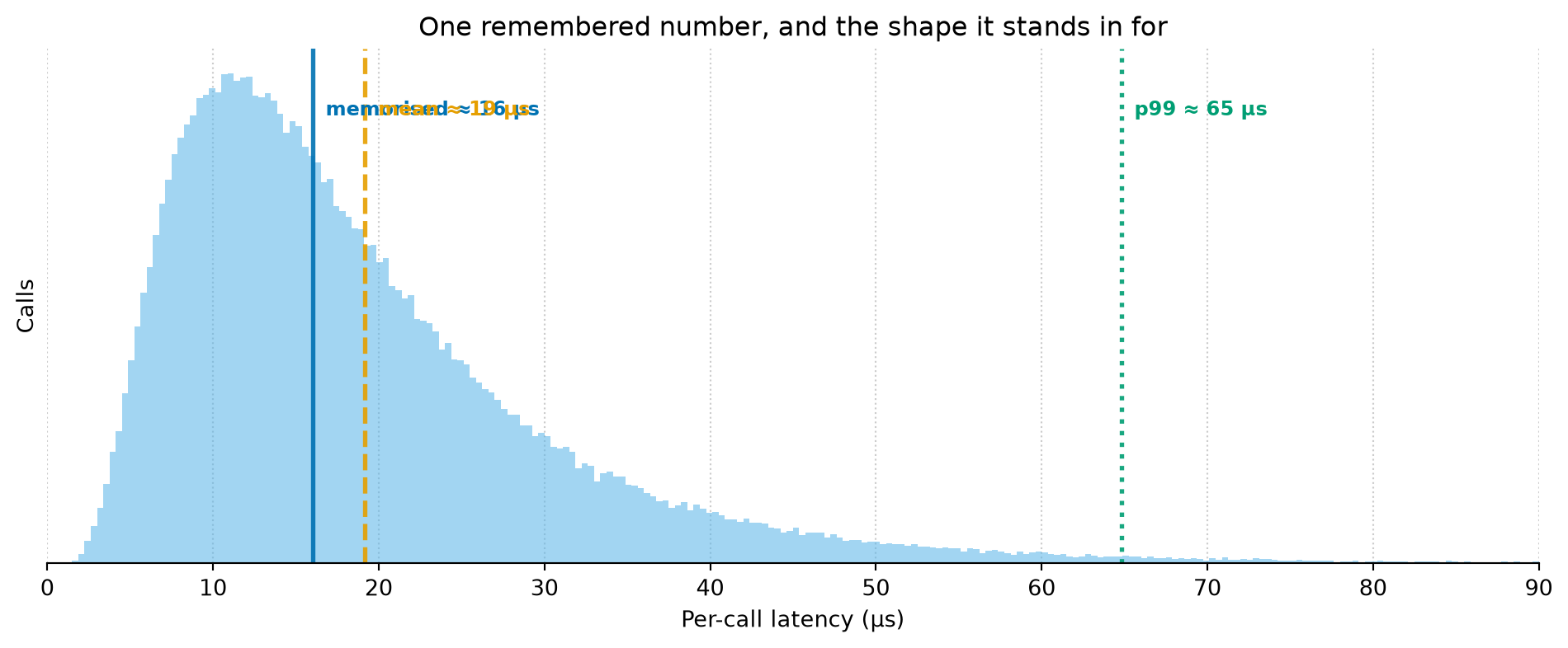
Figure 1: An illustrative distribution of per-call latency for an operation the table files under a single figure — here a random SSD read, textbook value ~16 µs. The memorised number sits near the peak, but the distribution is right-skewed: the mean is dragged higher by the tail, and the 99th percentile is several times the number you’d have quoted. The scalar you remember is one point on this shape, and it isn’t the point your latency budget is spent at.

I ran that expecting the memorised value to sit right on the peak, and it roughly did — what I sat with for a while was how far the tail ran past it. The mean is already a few microseconds to the right of the number I’d have quoted, dragged there by calls that queued or missed or got unlucky, and the 99th percentile is several times the textbook figure. The value I carry describes the calm middle of the operation. The tail, which is where the latency budget actually goes, isn’t in my head at all, because a single number has no room to keep it.

The number moved while I wasn’t looking

There’s a second thing the scalar can’t hold, and it’s the one Dan Luu’s needling really lands on. The table isn’t a snapshot of a distribution so much as a snapshot of a distribution that’s been sliding — and sliding at wildly different rates from one row to the next. Main-memory latency has barely moved in a decade; it was around a hundred nanoseconds then and it’s around a hundred nanoseconds now. Storage, meanwhile, moved by more than an order of magnitude: the SATA SSD that the older tables clocked at a couple of hundred microseconds became an NVMe drive an order of magnitude quicker, and the relationships I reason with shifted underneath me while the table in my head stayed still.

That’s the part I find unsettling, because the relationships are what I actually use. “Memory is a thousand times faster than disk” is the kind of thing I’ll say to justify a cache, and it was true for a particular year’s hardware. When the disk row moves an order of magnitude and the memory row doesn’t, the ratio — the thing I was really reasoning with — expires, and nothing tells me. Luu isn’t mostly saying the constants are wrong. He’s saying they’re old, and that “every programmer should know” them has kept them in circulation long after anyone last re-measured.

The snapshot I keep quoting

None of this makes the table useless, and I won’t stop using it — I’ll likely quote it again this week. The whole value of it is that it compresses a shifting, many-dimensioned distribution down to a number I can do arithmetic with in a supervision meeting, and that compression is the point, not a flaw: you cannot design against a histogram you’re holding in your head. But a lossy compression throws something away by definition, and this one throws away exactly two things — the spread, and the date. The figure you remember tells you neither how wide the operation’s tail runs nor how long ago the middle of it was true.

So I’ll keep the table, and what I’ve actually lost is smaller and more annoying than “the numbers are wrong”. It’s the ability to say, of any figure I’m quoting, when it last matched a real machine. I’ve caught myself sliding a “roughly” or a “ballpark” in front of the numbers, which sounds like statistical humility and is really just me not knowing which of them went off while I was still reciting them. Each entry has a best-before date printed in a font I can’t read, and I’ll go on quoting them anyway, at speed, in rooms where everyone nods.

---

Part of an occasional series reframing everyday engineering through a data scientist’s eyes. The ideas here are developed properly in Thinking in Uncertainty and Building with Certainty.