You already think in distributions

Percentiles, SLOs, error budgets: you’ve been doing distributional reasoning for years. Data science just gives you the tools to build the distributions yourself.

You don’t say “our API latency is 50ms”. Instead, you say “our p50 is 50ms and our p99 is 200ms”.

Those percentiles are distributional summaries. They tell you what’s typical, and they tell you how bad the tail gets. You report them because a single number, the average, hides too much. An average latency of 80ms could mean every request takes 80ms, or it could mean most take 20ms and a few take 500ms. Those are very different systems with very different problems, and the average can’t tell them apart.

That instinct, reaching for percentiles instead of averages, is distributional reasoning. The question is what follows from it.

SLOs are probability statements

“99.9% of requests complete in under 300ms” doesn’t describe what your system does; it’s a claim about the distribution of response times: specifically, that the 99.9th percentile sits below 300ms. The SLO (Service Level Objective) defines which part of the distribution you care about and where the threshold sits.

Error budgets make this explicit. If your SLO allows 0.1% of requests to exceed 300ms, you have a budget of acceptable failure. You can spend it on deployments, experiments, or planned maintenance. When a burn rate alert fires, you’re being told that the rate at which you’re consuming that budget has shifted. The distribution of outcomes has moved in a direction you care about.

This is, almost exactly, what data scientists call distributional drift: a change in the shape or location of a distribution over time. Your monitoring tools already detect it, but they just don’t call it that.

From consuming distributions to building them

The difference between what you do now and what data science asks you to do is narrower than it looks.

Your monitoring stack collects observations (request latencies, error counts, queue depths), computes distributional summaries (percentiles, rates, histograms), and alerts you when those summaries cross thresholds. You consume those distributions. Someone else (the team that built Prometheus, Datadog, Grafana) decided how to compute them.

Data science asks you to do the upstream part yourself. You start with raw observations, choose a model that describes how those observations are distributed, estimate its parameters from the data, and then use the fitted distribution to answer questions. The output is the same kind of thing you already work with: percentiles, tail probabilities, thresholds. But you’re constructing it rather than reading it off a dashboard.

Here’s an example that bridges the two worlds. Suppose you have a week of API response time data and you want to understand the distribution well enough to set an SLO.

import numpy as np
import matplotlib.pyplot as plt
from scipy import stats

rng = np.random.default_rng(42)

# Simulate a week of API response times (log-normal is typical for latencies)
log_mu = 3.9       # ~ 50ms median
log_sigma = 0.5
latencies = rng.lognormal(mean=log_mu, sigma=log_sigma, size=2000)

# Fit a log-normal distribution to the observations
shape, loc, scale = stats.lognorm.fit(latencies, floc=0)

# Compute percentiles from the fitted model
p50 = stats.lognorm.ppf(0.50, shape, loc, scale)
p95 = stats.lognorm.ppf(0.95, shape, loc, scale)
p99 = stats.lognorm.ppf(0.99, shape, loc, scale)

fig, ax = plt.subplots(figsize=(10, 5))
fig.patch.set_alpha(0)
ax.patch.set_alpha(0)

ax.hist(latencies, bins=60, density=True, alpha=0.6, color='#0072B2',
        edgecolor='white', linewidth=0.5)

x = np.linspace(0, latencies.max(), 500)
ax.plot(x, stats.lognorm.pdf(x, shape, loc, scale), color='#E69F00', linewidth=2,
        label='Fitted log-normal')

ymax = ax.get_ylim()[1]
for val, label, height in [(p50, 'p50', 0.92), (p95, 'p95', 0.82), (p99, 'p99', 0.72)]:
    ax.axvline(val, color='#D55E00', linewidth=1.5, linestyle='--', alpha=0.8)
    ax.text(val + 2, ymax * height, f'{label}: {val:.0f}ms',
            fontsize=9, color='#D55E00')

ax.set_xlabel('Response time (ms)')
ax.set_ylabel('Density')
ax.set_title('The same percentiles, built from a fitted model')
ax.spines['top'].set_visible(False)
ax.spines['right'].set_visible(False)
ax.yaxis.grid(True, linestyle=':', alpha=0.4, color='grey')
ax.set_axisbelow(True)
ax.legend(loc='upper right', framealpha=0.0)
plt.tight_layout()
plt.show()

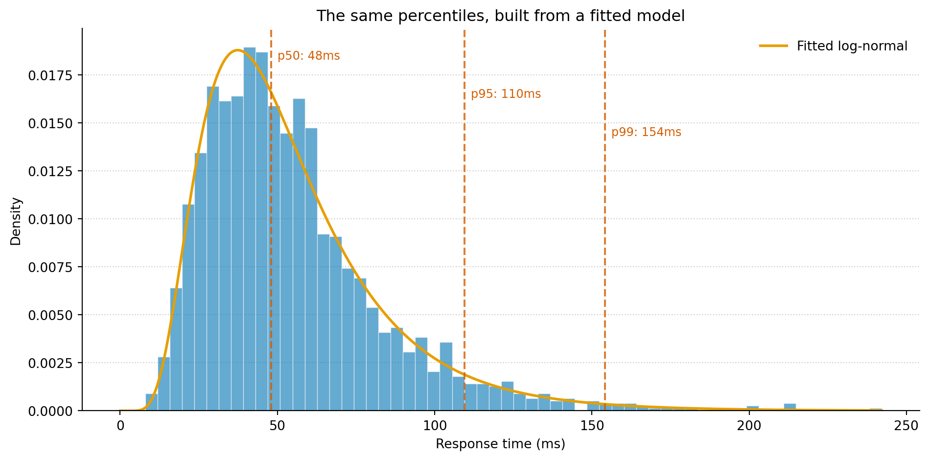
Figure 1: A histogram of observed latencies with a fitted log-normal distribution overlaid. The vertical lines mark the p50, p95, and p99 of the fitted model — the same quantities your monitoring dashboard reports, but derived from the model rather than read off a panel.

The histogram is the raw data. The orange curve is a fitted log-normal distribution: a model that describes the shape of the data with just two parameters. The dashed lines are percentiles derived from that model. These are the same numbers your monitoring dashboard would show you, except you built the distribution yourself from raw observations.

What a model buys you

Once you have a fitted distribution, you can answer questions the raw data can’t.

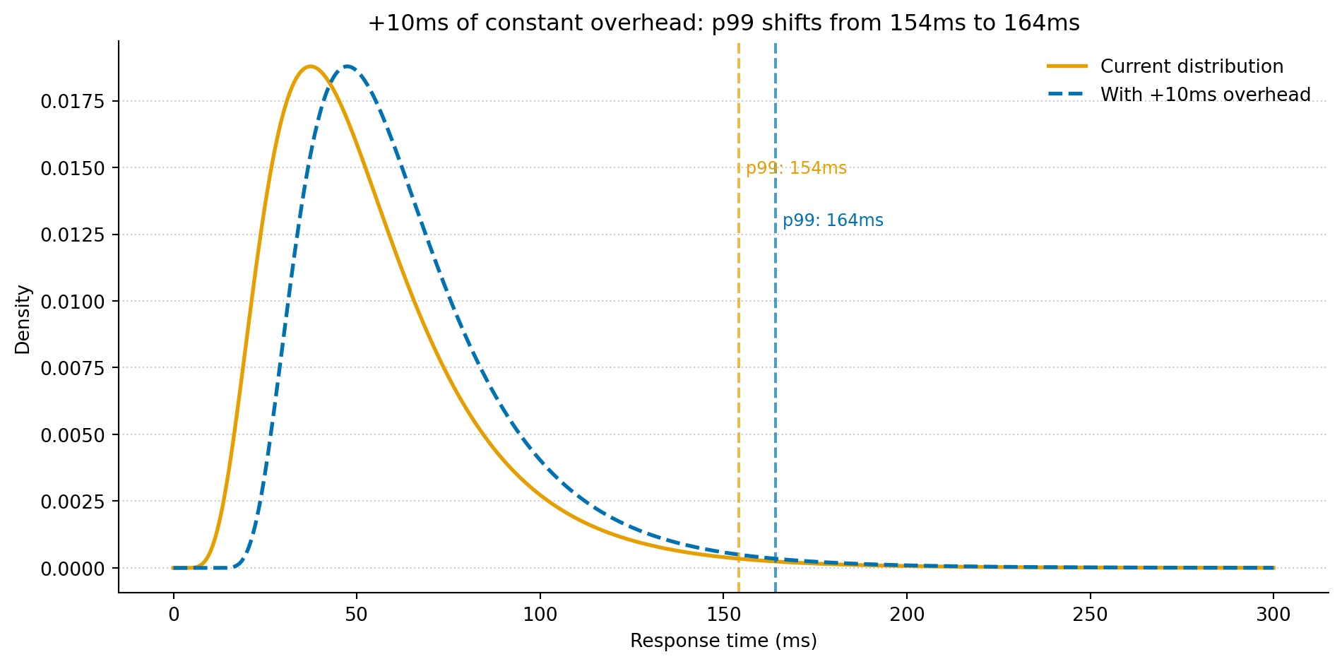
Your dashboard can tell you what the p99 was last week. A fitted model can tell you what the p99 would be if you added 10ms of constant overhead to every request, or if the spread of the distribution widened by 20%. You can simulate scenarios you haven’t observed yet and quantify the probability of outcomes that matter to you.

fig, ax = plt.subplots(figsize=(10, 5))
fig.patch.set_alpha(0)
ax.patch.set_alpha(0)

x = np.linspace(0, 300, 500)

# Current distribution
ax.plot(x, stats.lognorm.pdf(x, shape, loc, scale), color='#E69F00', linewidth=2,
        label='Current distribution')

# Shifted distribution (+10ms overhead)
shifted_p99 = stats.lognorm.ppf(0.99, shape, loc + 10, scale)
ax.plot(x, stats.lognorm.pdf(x, shape, loc + 10, scale), color='#0072B2', linewidth=2,
        linestyle='--', label='With +10ms overhead')

ymax = ax.get_ylim()[1]
ax.axvline(p99, color='#E69F00', linewidth=1.5, linestyle='--', alpha=0.7)
ax.text(p99 + 2, ymax * 0.75, f'p99: {p99:.0f}ms',
        fontsize=9, color='#E69F00')

ax.axvline(shifted_p99, color='#0072B2', linewidth=1.5, linestyle='--', alpha=0.7)
ax.text(shifted_p99 + 2, ymax * 0.65, f'p99: {shifted_p99:.0f}ms',
        fontsize=9, color='#0072B2')

ax.set_xlabel('Response time (ms)')
ax.set_ylabel('Density')
ax.set_title(f'+10ms of constant overhead: p99 shifts from {p99:.0f}ms to {shifted_p99:.0f}ms')
ax.spines['top'].set_visible(False)
ax.spines['right'].set_visible(False)
ax.yaxis.grid(True, linestyle=':', alpha=0.4, color='grey')
ax.set_axisbelow(True)
ax.legend(loc='upper right', framealpha=0.0)
plt.tight_layout()
plt.show()

Figure 2: The solid orange curve is the current fitted distribution. The dashed blue curve shifts it by 10ms, letting you ask: if we added a middleware layer with 10ms of constant overhead, what happens to our p99? The model says it moves from 154ms to 164ms — a useful first approximation before committing to a full load test.

That’s the payoff: you’ve gone from “what happened” to “what would happen if”. The model is a thinking tool, not just a summary. And the workflow — collect observations, fit a distribution, derive quantities you care about, simulate alternatives — is the same one that runs through most of applied data science.

Chaos engineering already got you here

If you’ve ever run a chaos engineering experiment — deliberately injecting failures to learn about system behaviour under stress — you’ve already accepted the core premise. You weren’t testing whether the system works. You were exploring the distribution of outcomes under adverse conditions: how often does the circuit breaker trip, how long do retries take, what’s the blast radius when a dependency goes down.

That’s distributional reasoning applied to systems. Data science applies it to data. The formalisms differ, but the underlying question is the same: given what I’ve observed under known conditions, what should I expect under different ones?

The shift is that you learn to construct these summaries yourself: for systems where no dashboard exists yet, using data where no SLO has been defined. The maths gets more formal. The thinking doesn’t change as much as you’d expect.

---

This article is part of a series drawn from Thinking in Uncertainty, a book that teaches data science to experienced software engineers.