Your model is wrong (and that’s the point)

Software engineers treat error as a bug, but in data science error is information. That shift changes everything.

Here’s something that runs through most of your working day without you noticing it:

assert f(x) == expected

Same input, same output, every time. If the assertion fails, something is broken, and you go fix it. Tests enforce this contract, CI gates on it, and the whole deployment pipeline assumes your code is deterministic. That instinct has served you well.

Now try this question: how many customers will visit our website tomorrow?

You can pull in historical traffic, adjust for day of the week, account for a marketing campaign, and the number you arrive at will still differ from what actually happens. This is not because the analysis was bad, but because the thing you’re measuring has real variability in it: tomorrow isn’t a rerun of today.

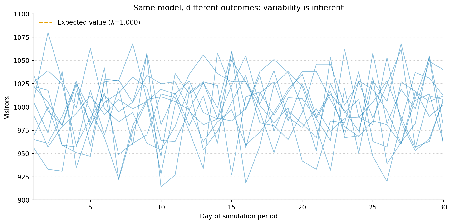
The code below simulates ten independent runs of a simple model (a Poisson distribution with an average of 1,000 visitors per day) over 30 days. Real traffic data are messier than this (overdispersed, autocorrelated, seasonal), but the Poisson keeps things simple enough to see the core point:

import numpy as np
import matplotlib.pyplot as plt

rng = np.random.default_rng(42)

fig, ax = plt.subplots(figsize=(10, 5))
fig.patch.set_alpha(0)
ax.patch.set_alpha(0)

days = np.arange(1, 31)
for _ in range(10):
    daily_visitors = rng.poisson(lam=1000, size=30)
    ax.plot(days, daily_visitors, alpha=0.45, linewidth=1, color='#0072B2')

ax.axhline(y=1000, color='#E69F00', linestyle='--', linewidth=1.5, alpha=1.0,
           label='Expected value (λ=1,000)')
ax.set_xlabel('Day of simulation period')
ax.set_ylabel('Visitors')
ax.set_title('Same model, different outcomes: variability is inherent')
ax.set_xlim(1, 30)
ax.set_ylim(900, 1100)
ax.yaxis.grid(True, linestyle=':', alpha=0.4, color='grey')
ax.set_axisbelow(True)
ax.spines['top'].set_visible(False)
ax.spines['right'].set_visible(False)
ax.legend(loc='upper left', framealpha=0.0)
plt.tight_layout()
plt.show()

Figure 1: Ten simulations from the same Poisson(λ=1,000) model over 30 days. Every trace used identical parameters; the variation between them is the model working correctly.

Every trace uses the same parameters. The dashed orange line marks the expected value, the long-run average that individual days scatter around. Look at how the ten traces wander apart despite identical settings. That spread is the model faithfully representing something true about the world: the process behind these numbers has genuine randomness in it.

The instinct you need to unlearn

You see a model that doesn’t match the observed outcome, and something in your brain says the model is wrong. In a deterministic system, that reaction is exactly right: residual error really does point to a bug. But when you’re working with data, a model that perfectly matches every observation is usually a sign of something worse.

It’s overfitting: memorising the quirks of one particular dataset instead of learning the pattern underneath. Think of it as the statistical equivalent of hard-coding a return value. It reproduces the training data exactly, but throw anything new at it and the whole thing falls apart.

In software engineering, passing tests means the system meets the specifications encoded in those tests, which is why tools like property-based testing exist: to probe whether your tests are actually telling you something meaningful. In data science, the equivalent suspicion fires when a model scores perfectly on its training data. A perfect training score usually means the model has mistaken noise for signal. When it meets data it hasn’t seen before (the real test), performance drops off a cliff.

Two kinds of error

Statisticians distinguish between reducible error and irreducible error. This distinction matters more than it sounds.

Reducible error is uncertainty you can shrink. Better features, more data, a more appropriate model structure. These all chip away at it. If your visitor-count model doesn’t account for day of the week, it will predict the same traffic on a Monday as on a Saturday. That’s reducible error: the information exists, and you haven’t used it yet.

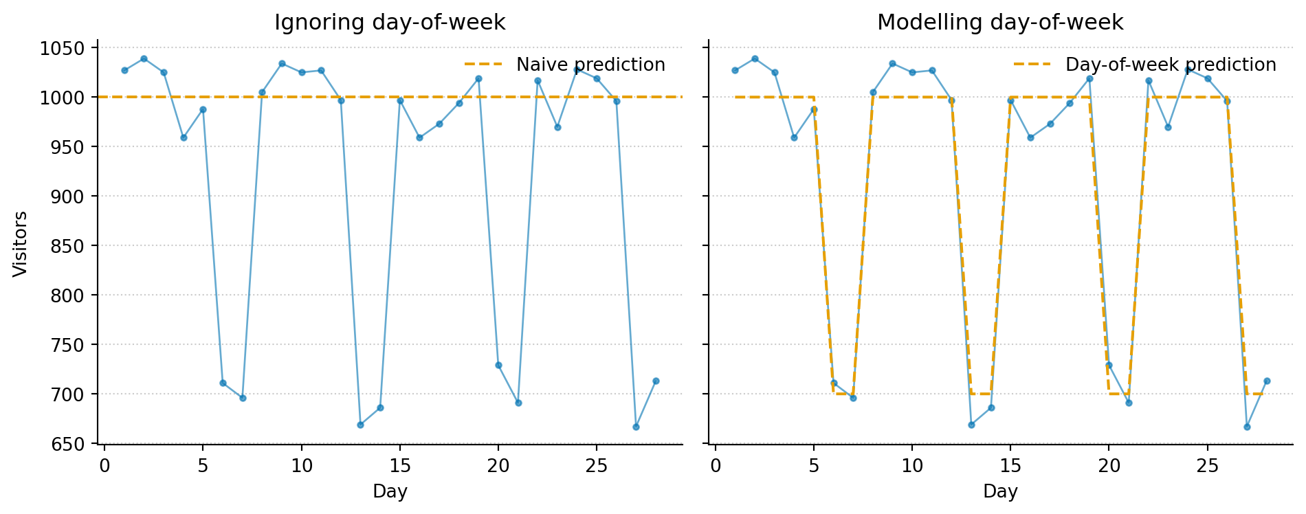
To make this concrete, here’s the same Poisson simulation with a twist. The first version ignores day-of-week effects entirely. The second builds them in: weekdays averaging 1,000 visitors, weekends averaging 700. Both have the same irreducible noise, but the second model explains more of the variation because it’s using information the first one throws away.

rng = np.random.default_rng(42)

days = np.arange(1, 29)  # 4 weeks
is_weekend = np.array([(d % 7) in (6, 0) for d in days])
lam_by_day = np.where(is_weekend, 700, 1000)

visitors = rng.poisson(lam=lam_by_day)

fig, (ax1, ax2) = plt.subplots(1, 2, figsize=(10, 4), sharey=True)
fig.patch.set_alpha(0)

# Left: naive model (ignores weekends)
ax1.plot(days, visitors, color='#0072B2', alpha=0.6, linewidth=1, marker='o', markersize=3)
ax1.axhline(y=1000, color='#E69F00', linestyle='--', linewidth=1.5,
            label='Naive prediction')
ax1.set_title('Ignoring day-of-week')
ax1.set_xlabel('Day')
ax1.set_ylabel('Visitors')
ax1.patch.set_alpha(0)
ax1.spines['top'].set_visible(False)
ax1.spines['right'].set_visible(False)
ax1.yaxis.grid(True, linestyle=':', alpha=0.4, color='grey')
ax1.set_axisbelow(True)
ax1.legend(loc='upper right', framealpha=0.0)

# Right: day-of-week model
ax2.plot(days, visitors, color='#0072B2', alpha=0.6, linewidth=1, marker='o', markersize=3)
ax2.plot(days, lam_by_day, color='#E69F00', linewidth=1.5, linestyle='--',
         label='Day-of-week prediction')
ax2.set_title('Modelling day-of-week')
ax2.set_xlabel('Day')
ax2.patch.set_alpha(0)
ax2.spines['top'].set_visible(False)
ax2.spines['right'].set_visible(False)
ax2.yaxis.grid(True, linestyle=':', alpha=0.4, color='grey')
ax2.set_axisbelow(True)
ax2.legend(loc='upper right', framealpha=0.0)

plt.tight_layout()
plt.show()

Figure 2: Accounting for day-of-week effects tightens the prediction around what actually happens. The remaining spread is irreducible: it’s the floor you can’t get below.

The day-of-week model is a better fit. Its predictions track the actual pattern more closely, and the residuals (the gaps between the orange line and the blue points) are smaller. But they don’t disappear. That remaining scatter is irreducible error: randomness baked into the process itself. No amount of additional data or cleverer modelling will eliminate it.

This is the part that takes adjusting to. Irreducible error isn’t a limitation of your model, it is simply your model telling you something true about the limits of what the data can reveal. A model that reports this honestly is more useful than one that pretends the noise isn’t there. The residual carries information: it tells you where prediction ends and genuine uncertainty begins.

Where this leads

Once error becomes something to read rather than something to fix, a cascade of things starts to look different. Residuals become a diagnostic tool: they are the first thing you check, not an afterthought. Model evaluation shifts from “how close is the fit?” to “is this model missing something structural?” And the question you’re really answering stops being “what will happen?” and becomes “what should I expect, and how confident should I be?”

That last question — how confident should I be — is one you’ve been answering your entire career. You just haven’t had to build the machinery yourself.

---

This article is part of a series drawn from Thinking in Uncertainty, a book that teaches data science to experienced software engineers.